Interferometers and resonators are photonic structures with many applications, including filtering, sensing, modulating, etc. They can be build in free-space, in optical fibers, or they can be integrated on a photonic integrated circuit. This simulation tool is mainly focused in the latter technology, but the theory is the same for all technologies, thus the simulations are valid in all contexts.
Integrated photonics
Integrated photonics is the technology that allows drawing circuits on the surface of a substrate, which can be a glass, a crystal, or a semiconductor. Using this technology, waveguides can be “drawn” through a chemical or physical process like etching, doping or depositing material following an arbitrary 2D pattern, called lithography. The main advantage is that once a lithographic mask is generated, it is easy to generate many copies of the same device using the same mask, as it used to be done in the past with lithographic paintings.
The main element needed for guiding the light is a waveguide, in particular, a waveguide that confines light vertically and horizontally. Confinement can be induced simply by having a so-called core with a higher refractive index, surrounded in all directions by a cladding, which is a material with lower refractive index so that light can undergo total internal reflection in the core. Some examples of materials used for integrated optics are doped glass, lithium niobate, and semiconductors such as GaAs, InP or silicon.
Simulating propagation through a waveguide
Before simulating the propagation of light through a waveguide, the actual waveguide mode has to be calculated. Examples of these calculations are provided in the fiber-optic mode calculator and in the planar waveguide calculator. The latter only provides the calculation of the mode confinement in the vertical direction, but not horizontally. To calculate the mode considering both confinements requires a mode solver software, although in some situations one can apply the effective index approximation to first solve the problem vertically and then use the calculated $n_{eff}$ values to solve the problem horizontally.
Once the effective index of the mode is calculated, it is easy to calculate how that mode propagates through a straight section, as the effective index dictates the phase velocity of the wave through the waveguide. If the waveguide propagates along the positive $z$ direction, the electric field propagates following this equation
\[\boldsymbol{E}(x,y,z) = \boldsymbol{E_0}(x,y)e^{ik_0 n_{eff} z}\]where $\boldsymbol{E_0}(x,y)$ is the mode profile vector, and $k_0$ is defined as:
\[k_0 = \frac{2\pi}{\lambda}\]where $\lambda$ is the wavelength in vacuum. We remind the reader that this way of modeling waves with complex numbers is very convenient for simplifying the math, although don’t forget that the actual electric field is the real part of that magnitude. To simplify the notation, we can just consider the electric field not as a vector 2D profile, but just a number that corresponds to the main electric field component at the maximum of the mode.
\[E(z) = E(0) e^{ik_0 n_{eff} z}\]This specific beam has no phase offset, if needed we can add a phase offset inside the complex exponential, but since phase can have an arbitrary offset, we can decide to set an offset equal to zero, and refer the phase of other beams with respect to this specific beam.
Simulating an interferometer
An interferometer is a device in which light is divided into two separate beams and then is recombined again. When the beams are recombined, one can apply the superposition principle by simply summing the electric fields of both beams (not the powers, but the electric field magnitudes). If the phase difference between both beams is zero, they constructively interfere generating a more powerful beam, while if the interference is destructive, the beam becomes weaker to the point of reaching zero output if the powers are balanced.
Let us assume the interferometer shown below, which called a Mach-Zehnder interferometer:
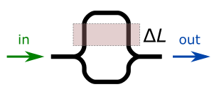
This specific case assumes symmetric 1x2 couplers, where symmetry imposes equal division of powers among the two branches. If the path lengths of each branch are $L_1$ and $L_2$, one simple way of calculating the output spectrum is just to sum the electric fields:
\[E_{MZI} = \frac{E_0}{2}\left(e^{ik_0 n_1 L_1}+e^{i k_0 n_2 L_2}\right)\]where $E_0$ is the input electric field, $n_1$ and $n_2$ the effective indices of branches 1 and 2, and $L_1$ and $L_2$ the length of each branch. therefore for calculating the transmission power coefficient we just have to square the absolute value of the electric field number E.:
\[T= {1\over 2} \left| e^{i k_0 n_1L_1}+e^{i k_0 n_2L_2}\right| ^2\]where $T$ is the transmitted energy. For cases in which the input and/or the output couplers of the interferometer are unbalanced (the splitting ratio is not 50%-50%), it is easy to calculate the response by weighting each branch differently.
The shape of this spectrum is a sinusoidal wave with a period called free-spectral range (FSR), which is equal to:
\[\Delta \lambda _{FSR} = \frac{\lambda_0 ^2}{n_{g1}L_1-n_{g2}L_2}\]Where $n_{g1}$ and $n_{g2}$ are the group indices of each branch, which would be the same if both branches have the same waveguide cross section. Remember that the group index is not the same as the effective index, as it refers not to the velocity of the phase front, but the velocity of the pulse envelope. It is defined as:
\[n_g=n_{eff}-\lambda\frac{dn_{eff}}{d\lambda}\]When the effective index is spectrally flat, the group index and effective index tend to the same value. However when the material has a higher dispersion or the waveguide is highly confining, there may be a large difference between those two numbers. For example, in a typical silicon-photonic waveguide with dimenstions 220x500nm, the effective index is close to 2.45 while the group index is 4.20, so in this case it is crucial not to confuse effective index with group index!
Simulating a ring resonator
A ring resonator is a resonator with the shape of a ring such as the one shown below:
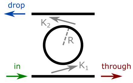
In this particular case, two couplers are connected to the ring, with cross-coupling energy coefficent $K_1$ and $K_2$. For example, if the input coupler couples 10% of the input energy into the ring after a single pass, then $K_1=0.1$.To calculate the drop and through spectra, one has to balance what comes into the resonator with what comes out. In this reference the problem is solved in detail:
\[T_{drop} =\frac{(1-r_1^2)(1-r_2^2)a}{1+(r_1 r_2 a)^2-2r_1r_2a \cos(\phi)}\] \[T_{through} =\frac{r_2^2 a^2-2r_1 r_2 a \cos(\phi)+r_1^2}{1+(r_1 r_2 a)^2-2r_1r_2a \cos(\phi)}\]where $T_{drop}$ and $T_{through}$ are the transmission energy coefficients that come out of the drop and through ports respectively, $r_1$, $r_2$ are the pass field coefficient of the couplers, and $a$ the field transmission coefficient after a single loop:
\(r_1= \sqrt{1-K_1}\) \(r_2 = \sqrt{1-K_2}\) \(a = \sqrt{A}\)
where $K_1$, $K_2$ were defined previously, and $A$ is the transmission energy coefficient (equal to one if attenuation is neglected).
Finally, $\phi$ is the phase shift after a single loop through the ring: \(\phi = \frac{2\pi}{\lambda_0}n_{eff}L\)
where $L$ is the perimeter length of the ring. The spectra of a ring resonator, instead of being a sinusoidal wave as for the interferometer, consists of a series of peaks which can be approximated to a lorentzian shape (except for very high coupling conditions). The spectral separation between peaks is also known as free-spectral range, and has the same expression as for the interferometer, substituting the length difference with the ring length:
\[\Delta \lambda _{FSR} = \frac{\lambda_0 ^2}{n_g L}\]On the other hand, the width of the peaks can be also calculated analytically as shown in this reference:
\[\Delta \lambda_{FWHM} \approx \frac{(1-r_1 r_2 a)\lambda_{res} ^2}{\pi n_g L \sqrt{r_1 r_2 a}}\]where FWHM stands for full-width at half-maximum which is the spectral width of the peak at half its intensity, and $\lambda_{res}$ is the resonance wavelength. This approximation is only valid in cases where the width is narrow as compared to the FSR. When coupling coefficients become very high (>50%) or loss is very high, then this equation is not precise anymore.
Other useful parameters which are very common in any kind of resonator are the Finesse ($F$), defined as:
\[F = \frac{\Delta \lambda _{FSR}}{\Delta \lambda_{FWHM}}\]which indicates the number of loops the light undergoes before leaving the resonator, and the quality factor ($Q$) defined as:
\[Q = \frac{\lambda_{res}}{\Delta \lambda_{FWHM}}\]which indicates the number of oscillations light undergoes before leaving the resonator.
This applet
This applet calculates the transmission spectra of Mach-Zehnder interferometers and ring resonators. For interferometers, the user can tweak the path difference, the effective index, the temperature, the wavelength constraints, and the dispersion through the parameter $n_g - n_{eff}$. The reason for using that as a parameter instead of directly $n_g$ is to get a more realistic change when $n_{eff}$ is changed. In realistic situations, when $n_{eff}$ varies as a consequence of an extrinsic parameter like a chemical concentration or a temperature change, $n_g$ also changes by the same amount in first approximation. For that reason it is more intuitive to use $n_g - n_{eff}$ as a fixed parameter that depends on the waveguide dispersion.
Under the Ring resonator tab, the program calculates both the through and the drop spectra changing the ring radius, effective index, temperature, and coupling coefficient. The program solves the equations for the specific case of $A$=1 (negligible absorption in the ring) and $K_1$ = $K_2$ (symmetric couplers). Under these conditions, the resonance peaks have maximum visibility (critical coupling condition).
Some examples for the user to try:
-
A Si-photonic waveguide buried in silica with standard dimensions 220x500nm, has the following parameters at 1.55 $\mu m$: $n_{eff}$ = 2.45, $n_g$ = 4.20, thus $n_g-n_{eff} = 1.75$; $dn_{eff}/dT = 1.8 · 10^{-4} K^{-1}$.
-
A silica waveguide: $n_{eff} \approx 1.45$; $n_g \approx 1.465$, thus $n_g-n_{eff} \approx 0.015$; $dn_{eff}/dT = 1.05 · 10^{-5} K^{-1}$
It is worth playing with the $\Delta L$ (for MZIs) or $R$ (for rings) parameter, to see how much the fringes or peaks shift for small changes. It will become obvious to the user to realize how difficult it is to predict the absolute position of the fringe or the ring peak when this structure is manufactured. FSRs are easy to predict, but absolute peak positions are phase-sentitive, therefore when a filter is needed at a certain wavelength, what people usually do is to introduce a phase shifter within the structure (with a heater or with any other index-changing mechanism) and do the fine tuning afterwards.
The applet should appear below; I hope you will find it useful. If you do please spread the voice, and if you use it in a published document please cite the website. And if you find any mistake or want to propose some improvement, please contact me!