Light propagating in multilayered media is not difficult to simulate by using the transfer matrix method. This method assigns matrices to layers and/or interfaces and calculates electromagnetic propagation by matrix-multiplying from the first element to the last. Actually, there are two possible transfer-matrix methods to solve a multilayer problem. In one method, which the one used used in Born & Wolf famous book, the vector propagated is the total electric and magnetic fields. Using the continuity equations for electromagnetic waves, one can assign just one matrix to each layer, and the job is done. Another method, which is more intutive, propagates the magnitudes of the electric fields propagating to the left and to the right. It is the method used, for example, in Yeh’s book. This way, apart from the matrix required for the propagation through every layer, every interface also requires a matrix which contains the Fresnel coefficients of reflection and transmission. The main disadvantage of this method is that it requires two matrices per layer. However, this method, being more intuitive as the scattering and propagation matrix are distinct, makes it more convenient to generalize the problem to other situations, therefore this is the one we will apply.
Let us first assume a plane. We will consider the electric field as a complex numbers whose phase tells us about the phase of the wave. Of course, the real electric field of the wave is only the real part of this magnitude, but considering the complex number simplifies the calculations as trigonometric functions become exponentials, which are easier to handle. Assuming that the plane wave wave propagates in the positive $z$ direction through a medium with refractive index $n$, at an angle $\theta$ with respect to the $z$ axis, the magnitude of the electric field can be described as:
\[E^{+}(z) = E^{+}(0)e^{ik_zz}\]where $E^{+}$ means electric field of the wave propagating in the forward direction, and $k_z$ is the $z$ component of the propagating constant, which is equal to
\[k_z = k_0n \cos(\theta) = \frac{2\pi}{\lambda_0}n\cos(\theta)\]if the wave propagates in the backwards direction (towards negative $z$), the equation would have an opposite sign on k:
\[E^{-}(z) = E^{-}(0)e^{-ik_zz}\]where $E^{-}$ represents the field propagating backwards (towards negative $z$).
Propagation matrix
We can use matrices to calculate waves along $z$ propagating simultaneously in both directions. If a layer has a thickness $d$:
\[E^{+}(d) = E^{+}(0)e^{ik_zd}\] \[E^{-}(d) = E^{-}(0)e^{-ik_zd}\]or in matrix form:
\[\begin{pmatrix} E^{+}(d)\\ E^{-}(d) \end{pmatrix} = \begin{pmatrix} e^{ik_zd}&0\\ 0&e^{-ik_zd} \end{pmatrix} \begin{pmatrix} E^{+}(0)\\ E^{-}(0) \end{pmatrix}\]since we want the subsequent matrix multiplications to be inserted on the right, let’s invert the terms:
\[\begin{pmatrix} E^{+}(0)\\ E^{-}(0) \end{pmatrix} = \begin{pmatrix} e^{-ik_zd}&0\\ 0&e^{ik_zd} \end{pmatrix} \begin{pmatrix} E^{+}(d)\\ E^{-}(d) \end{pmatrix}\]and we now define our transfer matrix for this specific layer with thickness $d$ and index $n$ as:
\[\boldsymbol{T}^{(prop)} = \begin{pmatrix} e^{-ik_zd}&0\\ 0&e^{ik_zd} \end{pmatrix} = \begin{pmatrix} e^{-ik_0 d n \cos{\theta}}&0\\ 0&e^{ik_0 d n \cos{\theta}} \end{pmatrix}\]Interface matrix
Now let us calculate the matrix to be inserted at every interface. Let us assume an interface between media 1 and 2, with indices $n_1$ and $n_2$. Let us assign a sign convention as shown in the following figure:
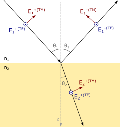
where we show both polarizations, which we call TE and TM. TE (transverse-electric) polarization, also known as $s$-polarization, refers to the case where the electric field is parallel to the surface, for any incidence angle. That’s why in the figure is represented by a vector pointing perpendicularly to the screen. TM (transverse-magnetic) polarization, also known as $p$-polarization, refers to the case where the magnetic field of the wave is parallel to the interface. This means that the electric field is not parallel for incidence angles greater than zero, and it changes direction upon reflection or refraction. It is also worth noting that for normal incidence, even though TE and TM converge to the same case, there is a sign change in the reflectivity coefficient between both cases, as the vector points to the opposite direction.
Let us now calculate the reflection and transmission coefficients. For this, we will use the Fresnel equations, which can be deduced from continuity conditions of electromagnetic fields in interfaces, and are shown below:
\[r_{12}^{(TE)}=\frac{n_{1}\cos\theta _{1}-n_{2}\cos\theta _{2}}{n_{1}\cos\theta _{1}+n_{2}\cos\theta _{2}}\] \[t_{12}^{(TE)}=\frac{2n_{1}\cos\theta _{1}}{n_{1}\cos\theta _{1}+n_{2}\cos\theta _{2}}\] \[r_{12}^{(TM)}=\frac{n_{2}\cos\theta _{1}-n_{1}\cos\theta _{2}}{n_{2}\cos\theta _{1}+n_{1}\cos\theta _{2}}\] \[t_{12}^{(TM)}=\frac{2n_{1}\cos\theta _{1}}{n_{2}\cos\theta _{1}+n_{1}\cos\theta _{2}}\]where $r_{12}^{(TE)}$ and $t_{12}^{(TE)}$ are the reflection and transmission complex coefficients from medium 1 to medium 2 for TE polarization. On the other hand, $r_{12}^{(TM)}$ and $r_{12}^{(TM)}$ are the coefficients for the TM polarization. The angles $\theta_1$ and $\theta_2$ are the angles of propagation in media 1 and 2 respectively with respect to normal of the interface; these are related by Snell’s law:
\[n_1 \sin \theta_1 = n_2 \sin \theta_2\]The Fresnel coefficients can be simplified defining a new variable called $\gamma$:
\[r_{12}=\frac{\gamma_1-\gamma_2}{\gamma_1+\gamma_2}\] \[t_{12}=\frac{2\gamma_1}{\gamma_1+\gamma_2}\\\]where the definition of $\gamma$ depends on the polarization. For the $i$-th layer with refractive index $n_i$ and angle $\theta_i$:
\[\gamma_i^{(TE)}=n_i\cos \theta_i\] \[\gamma_i^{(TM)}=\frac{cos \theta_i}{n_i}\\\]With these equations we can now calculate the transfer matrix corresponding to the interface between the two media. When waves come from the left and right side of the interface, the output waves can be calculated from the scattering matrix:
\[\begin{pmatrix} E_1^{-}\\ E_2^{+} \end{pmatrix} = \begin{pmatrix} r_{12}&t_{21}\\ t_{12}&r_{21} \end{pmatrix} \begin{pmatrix} E_1^{+}\\ E_2^{-} \end{pmatrix}\]This can be reordered to generate a transfer matrix, which relates the fields on the left and right sides of the interface:
\[\begin{pmatrix} E_1^{+}\\ E_1^{-} \end{pmatrix} = \begin{pmatrix} \cfrac{1}{t_{12}} & -\cfrac{r_{21}}{t_{12}}\\ \cfrac{r_{12}}{t_{12}} & t_{21}-\cfrac{r_{12}}{t_{12}}r_{21} \end{pmatrix} \begin{pmatrix} E_2^{+}\\ E_2^{-} \end{pmatrix}\]This can be simplified by applying the symmetry relations of the Fresnel coefficients (obtained when exchanging medium 1 and 2), which are:
\[r_{12}=-r_{21}\] \[t_{12}t_{21}-r_{12}r_{21}=1\]This yields a simpler transfer matrix equation for the interface:
\[\begin{pmatrix} E_1^{+}\\ E_1^{-} \end{pmatrix} = \frac{1}{t_{12}} \begin{pmatrix} 1 & r_{12}\\ r_{12} & 1 \end{pmatrix} \begin{pmatrix} E_2^{+}\\ E_2^{-} \end{pmatrix}\]where the transfer matrix becomes:
\[\boldsymbol{T}_{12}^{(int)} = \cfrac{1}{t_{12}} \begin{pmatrix} 1 & r_{12}\\ r_{12} & 1 \end{pmatrix}\]where $(int)$ denotes an interface transfer matrix. Substituting the Fresnel coefficients, and after some algebraic manipulation, the resulting matrix becomes:
\[\boldsymbol{T}_{12}^{(int)} = \frac{1}{2} \begin{pmatrix} 1 + \cfrac{\gamma_2}{\gamma_1}& 1-\cfrac{\gamma_2}{\gamma_1}\\ 1-\cfrac{\gamma_2}{\gamma_1} & 1 + \cfrac{\gamma_2}{\gamma_1} \end{pmatrix}\]where $\gamma$ was defined above for each polarization.
It is worth noting that the magnitude $n \cos \theta$ appears very often (it is $\gamma^{(TE)}$ and it is also used in the propagation matrix); we can calculate it for every layer as a function of the incident angle on the very first layer, as the angles of propagation do not depend on what layers are in the middle, because all interfaces are parallel. For any $i$-th layer with refractive index $n_i$ and angle $\theta_i$, it is easy to demonstrate from Snell’s law the following property:
\[n_i\cos\theta_i = \sqrt{n_i^2-n_0^2 \sin^2 \theta_0}\]where $n_0$ and $\theta_0$ are the refractive index and propagation angle of the very first medium where the incident light is coming.
Multilayer calculation
Now that we have the transfer matrix of the propagation through a single layer, and the transfer matrix of an arbitrary interface, we can calculate a multilayer by just stacking matrix multiplications considering all layers and interfaces:
\[\begin{pmatrix} E_{0}^{+}\\ E_{0}^{-} \end{pmatrix} = \boldsymbol{T}_{01}^{(int)} \boldsymbol{T}_{1}^{(prop)} \boldsymbol{T}_{12}^{(int)} \boldsymbol{T}_{2}^{(prop)} ... \boldsymbol{T}_{(N-2) (N-1)}^{(int)} \boldsymbol{T}_{N-1}^{(prop)} \boldsymbol{T}_{(N-1) N}^{(int)} \begin{pmatrix} E_{N}^{+}\\ E_{N}^{-} \end{pmatrix} = \boldsymbol{T_{0N}} \begin{pmatrix} E_{N}^{+}\\ E_{N}^{-} \end{pmatrix}\]So now, to calculate the the transmission and reflection coefficients of the whole multilayer system when illuminated from the left side, we set the input from the right equal to zero:
\[\begin{pmatrix} E_{0}^{+}\\ E_{0}^{-} \end{pmatrix} = \begin{pmatrix} t_{11}&t_{12}\\ t_{21}&t_{22} \end{pmatrix} \begin{pmatrix} E_{N}^{+}\\ 0 \end{pmatrix}\]and we then extract the ratios:
\[r = \frac{E_{0}^{-}}{E_{0}^{+}} = \frac{t_{21}}{t_{11}}\] \[t = \frac{E_{N}^{+}}{E_{0}^{+}} = \frac{1}{t_{11}}\]These coefficients are the complex terms; to extract the energy coefficients (reflectance and transmittance) we can apply these equations, obtained from the ratios of the Poynting vectors.
\[R = |r|^2\] \[T = \frac{Re(n_N\cos\theta_N)}{Re(n_0\cos\theta_0)}|t|^2\]where we introduced the real parts of the $k$-vectors to consider the case of total internal reflection, in which the propagation angle is imaginary and the transmission becomes zero.
This method is valid for any set of layers. A computer program which implements this method can be used to simulate single layers, Fabry-Perot resonators, periodic systems like distributed Bragg reflectors (DBRs), etc.
Absorption or loss
The formalism used assumed that the materials forming the multilayer were lossless. However, introducing an absorption or loss coefficient in the system is straightforward. One has just to consider instead of a real refractive index, a complex one:
\[\tilde{n} = n + i \kappa\]By doing so, when we substitute the plane wave equation shown above, the result is:
\[E^{+}(z) = E^{+}(0)e^{i k_0 (n + i\kappa) z} = E^{+}(0)e^{- k_0 \kappa z} e^{i k_0 n z}\]To understand the relationship of the imaginary part of the refractive index with the loss coefficient of the material, we have to remember Beer’s law:
\[I(z)=I(0)e^{-\alpha z}\]which establishes an exponential decay of the intensity of the light $I$ along a material with a loss coefficient $\alpha$. As the light intensity is proportional to the square of the electric field, we can now relate the imaginary part of the refractive index with the loss coefficient:
\[\kappa = \frac{\alpha}{2 k_0} = \frac{\alpha \lambda}{4 \pi}\]This means that introducing loss into the calculation is as simple as assigning an imaginary part to the refractive index of the material, without having to change anything else in our solver. The imaginary part in the refractive index will also alter the Fresnel coefficients at the interface, which is why a metal has such a high reflectivity coefficient. This means we can even simulate metal layers in our system without having to change anything in the program.
Interactive applet for multilayer calculation
Below there is an implementation of the method for a set of single layers, or to a periodic arrangement of pairs of layers A and B. The user can change the thickness and the refractive index of each layer, the refractive indices of the incident and final materials, the incidence angle, and the wavelength range.
We encourage the user to play with the parameters to see the effects of changing each magnitude. As examples, we propose some ideas to play with:
-
Try to design an anti-reflection coating for a silicon solar cell (refractive index of silicon is $\approx$3.9 in the visible).
-
In the periodic Bragg mirror, play with the index contrast, how does it affect the reflection spectrum? What about the effect of the duty cycle?
-
What happens to the spectrum when the incident angle changes?
The applet should appear below (if it doesn’t please contact me).
Bibliography
-
M. Born and E. Wolf, “Principles of Optics”, 6th edition, Cambridge University Press (1986).
-
P. Yeh, “Optical Waves in Layered Media”, Ed. John Wiley and Sons, (1988).