This applet is called FIMOC (fiber-optic mode online calculator). With it you will be able to calculate and visualize the propagating modes of any step-index fiber of your choice.
If you want to go directly to the software, scroll to the bottom, but if you are interested in where these modes come from, read on.
Optical fibers
Did you know that light in optical fibers follow the same patterns as the mechanical vibrations of a drum? In the next sections, we’ll see why. Let’s start from the beginning. Optical fibers are long cylinders of transparent glass or plastic, which are characterized by having a refractive index variation along its radial direction. The central region is called the core of the fiber, while the external one is called the cladding, which is typically made of the same material with a different doping concentration. In general, the core region has a higher refractive index that the cladding, because light hitting an interface from higher to lower index can undergo total internal reflection, which is a necessary condition for guiding, or at least for guiding with a reasonable loss value.
A very typical type of fiber is called the step-index fiber, which has constant refractive index values at the core and cladding:
\[n(r)= \left\{ \begin{array}{ll} n_{core} & r\le a \\ n_{clad} & r>a \end{array} \right.\]where $a$ is the radius of the core, and $n_{core}$ and $n_{clad}$ are the indices of the core and the cladding, respectively. The radius of the cladding doesn’t really matter much, because guided light cannot propagate along the cladding, it rapidly decays along the first few microns of cladding, so to simplify the problem, we can consider the cladding radius to be infinite.
Numerical aperture
A very important parameter of a fiber is its numerical aperture, which is a number that tells you about its acceptance angle when coupling light from outside. Precisely, it is equal to the sine of the half-angle of the acceptance cone. If you want the light to be confined in the core, you have to couple the light so that when it propagates in the core within the fiber’s critical angle. In a step-index fiber, you can easily calculate (by applying Snell’s law) how much this angle should be (within the ray-optics approximation, which is quite valid for multimode fibers), so the numerical aperture of the fiber turns out to be:
\[\text{NA} = \sqrt{n_{core}^2-n_{clad}^2}\](you can find a demonstration here for instance). When you buy a fiber, the datasheet will most likely report the numerical aperture of the fiber, which tells you not only about the collecting (or emitting) angle of the fiber but also about the fiber’s index contrast, so remember this definition, as we will need this parameter later on.
Another information you will find about the fiber you are considering to buy is whether the fiber is single-mode or multi-mode. Modes? What are you talking about?? Bear with me, things will now get more interesting.
Electromagnetic wave equations
When light propagates in the fiber, geometrical optics and the critical angle concept provides a very useful picture, but when things get small, geometrical optics fails to provide a precise model. If you want the full picture you need to solve the actual electromagnetic wave equations, so that’s what we will do now. Beware, there’s some math ahead, but don’t be scared, you don’t really have to understand every single equation, I just want you to have all the details in case you are interested, but feel free to skip this section if you feel overwhelmed.
So let’s start at the beginning. When light propagates through a medium with a refractive index function $n(\vec{r})$, any of the components of the electric or magnetic field follows the so-called Helmholtz’s equation [1]:
\[\nabla^2 U + n^2(\vec{r})k_0^2 U=0\]where $n$ is the refractive index and $k_0=2\pi/\lambda_0$, being $\lambda_0$ the wavelength in vacuum.
Now let us assume that our medium has cylindrical symmetry. That means that it is convenient to apply Helmholtz’s equation in cylindrical coordinates:
\[\frac{\partial^2U}{\partial r^2}+\frac{1}{r}\frac{\partial U}{\partial r}+\frac{1}{r^2}\frac{\partial ^2U}{\partial\phi ^2}+\frac{\partial ^2U}{\partial z^2}+n(r)^2k_0^2U=0\]To solve this equation in 3D let’s try with a trial solution separating the variables:
\[U(r,\phi,z)=u(r)e^{-jl\phi}e^{-j\beta z} \quad \text{for} \: l=0,\pm 1,\pm 2...\]where $\beta$ is the propagating constant along $z$ and the integer number $l$ represents the azimutal dependence of the mode: when $l=0$, it does not depend on the azimut angle $\phi$, and when $l\ne0$, you can imagine the 2D mode as a cake subdivided by cuts through its center, so $l$ is simply the number of cuts.
When we substitute this differential equation in the previous expression, we get:
\[\frac{d^2u}{dr^2}+\frac{1}{r}\frac{du}{dr}+\left(n^2(r)k_0^2-\beta^2-\frac{l^2}{r^2}\right)u=0\]which is the differential equation we have to solve for the specific radial index profile of our fiber.
The differential equation shown before can have many solutions. Every solution is called a mode, which is represented by the 2D profile of the electromagnetic fields that can propagate through the fiber satisfying the boundary conditions. Same happens for example with vibration modes of a string under tension, each vibration harmonic is a mode. In our case, for every $l$ parameter, you may find zero, one, or many possible modes, each one characterized by a different propagation constant $\beta$. Some fibers have a single propagating mode in total, which are called single-mode fibers, and some have more than one mode, which are called, what a surprise, multimode fibers.
Solution for step-index fibers
So the case we are going to solve is the step-index fiber, which we previously defined. The good news is that this equation has analytic solution, which is:
\[u(r) = \left\{ \begin{array}{ll} J_l(k_T r) & r\le a \\ K_l(\gamma r) & r>a \end{array} \right.\]where $k_T$ and $\gamma$ are defined as:
\[k_T^2=n_{core}^2k_0^2-\beta^2\] \[\gamma^2=\beta^2-n_{clad}^2k_0^2\]and J and K are the Bessel functions of the first and the modified second kind respectively. If it’s the first time you hear about Bessel functions don’t panic, they are functions that appear very often as solutions to differential equations in cylindrical or spherical coordinates, and many scientific calculators or numerical packages have them in their arsenal. You can simply consider the Bessel functions of the first kind as oscillating functions with a decaying amplitude, and the ones of the modified second kind as some kind of decaying stretched exponential. They look like this:
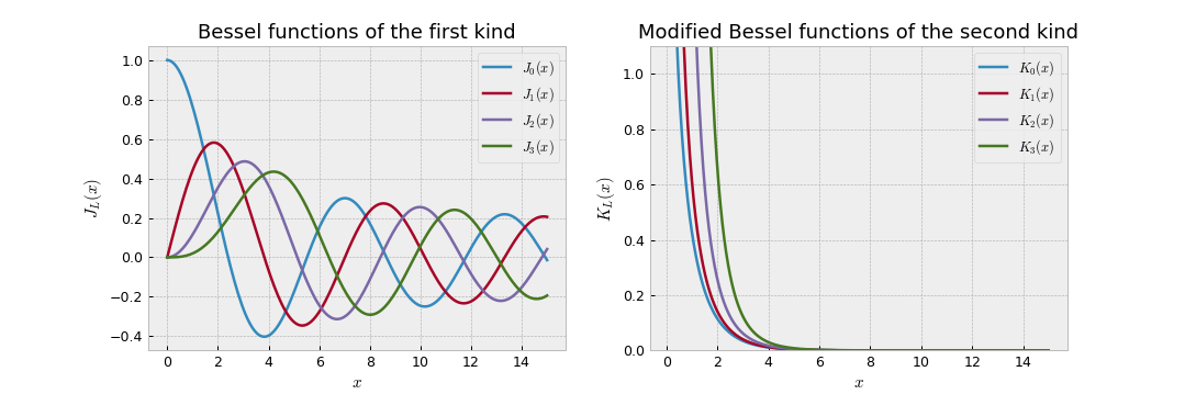
Bessel functions of the first kind J and modified second kind K
Actually, the Bessel functions of the first kind are the solutions of the mechanical vibration of a drum with a circular shape, as shown here. The only difference with the fiber-optic case is that the decay at the edges is abrupt for the drum case, and is gradual with a modified Bessel function in the fiber-optic case, but in the core all the modes follow the same mathematical function.
So you may think that we have found the solution, so we can all go home, but unfortunately we are not done yet. We still need to calculate the propagation constant and the actual electric and magnetic field components that satisfy the boundary conditions, and that is not straightforward in the general case. However in realistic fibers, we can make an aproximation which will simplify the task.
Linearly polarized (LP) modes
Most fibers in the real world have a weak refractive index contrast ($n_{core}-n_{clad}«1$), which is called weakly guiding condition. In this approximation, the boundary conditions at the interface can be simplified so that both electric and magnetic fields are continuous and derivable at $r=a$. This greatly simplifies the calculation of the modes, although the solution of the actual propagation constants is not analytical but has to be calculated numerically. Once we get the scalar function $u(r)$, the small index contrast allows us to apply the $u(r)$ profile to any electric field component to get the actual electric field profiles for each polarization, which we choose vertical and horizontal for convencience. Thus in this approximation, each LP mode actually corresponds to two differently polazired modes, one vertical and one horizontal, with identical mode profiles and propagating properties.
So this program numerically calculates all possible solutions that satisfy the boundary conditions, and computes the mode profiles for each case. But how many modes does a certain fiber have? To answer that question, it is very helpful to define some new variables (don’t worry, we’re almost there, I promise). First let us define a normalized adimensional parameter called the $V$-number or the $V$-parameter of the fiber:
\[V=2\pi\frac{a}{\lambda_0}\text{NA}\]This number is very important because it is a single number that can tell you about the number of modes the fiber can hold at a certain wavelength.
In the following plot you can see how many modes there are as a function of the $V$ number.
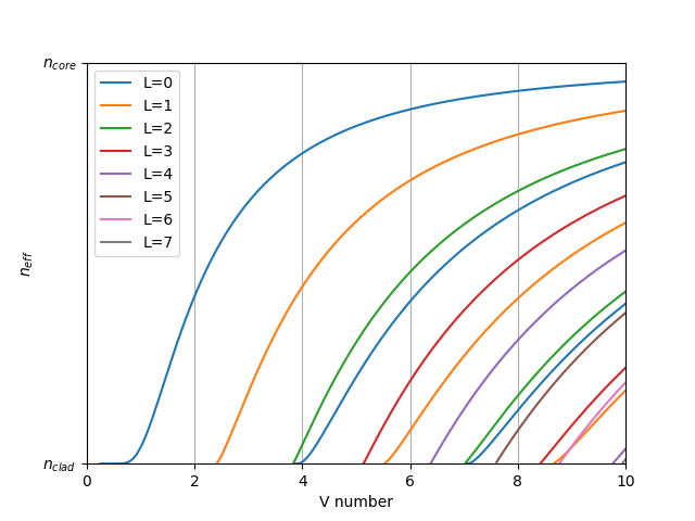
Calculated modes vs. V-number.
When V < 2.405, the fiber only has one mode (it is a single-mode fiber). Beyond V=2.405, a higher-order mode emerges. That means that V=2.405 is called the cut-off of the higher order mode, below which that mode cannot propagate. Every high-order-mode has a cut-off, but the first cut-off is the most important because it determines whether the fiber is single-mode or multimode.
It is worth noting that the V-number, thus the single- or multi-mode condition, not only depends on the fiber geometrical properties, but also on the wavelength. So a single-mode fiber always becomes multimode at some shorter wavelength.
You may notice that the fundamental mode has no cut-off, does it mean that a fiber can guide any wavelength? Mathematically, yes, but in practice no, because some approximations fall apart when guiding becomes extremely weak (V « 1). In particular, when V«1:
- bending loss becomes extremely high (even for very smooth curves)
- the radius of the cladding becomes important, as the evanescent field in the cladding can reach very far, making the infinite cladding approximation invalid.
- silica glass absorbs wavelengths above $\gtrsim 2 \mu$m anyway.
Now that we understand the mode cut-offs let’s see how LP modes look like. They are characterized by two parameters, the $l$ parameter, as we defined before (the number of cuts on the cake through its center), and a second parameter $m$ which is the number of zeros when going along the radial direction:
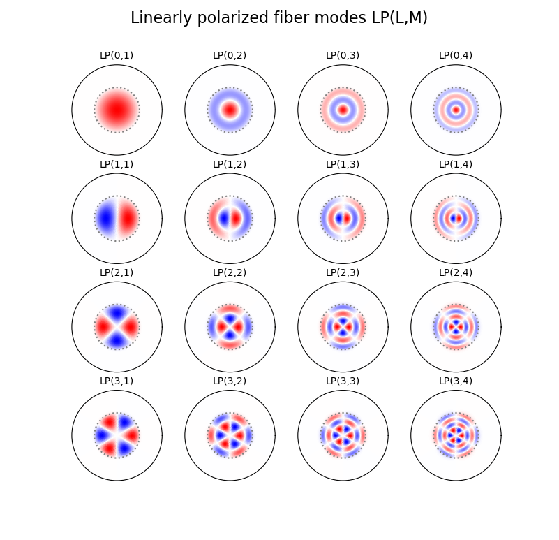
Example of some LP modes in a typical multimode fiber. Red and blue colors represent electric fields with opposite signs.
Number of modes
It is worth mentioning that every LP mode can actually represent more than one propagating mode. Let’s remember that each mode can have two polarizations (like the vibrations of a string, by the way), which in the low-index-contrast approximation they can be considered as degenerate. But when $\lvert l\rvert$>0, the mode also has two helical polarities, corresponding to $+l$ and $-l$. This means that modes with $l$=0 have a degeneracy of 2 while modes with $\lvert l \rvert$>0 have degeneracy 4. However they are not typically represented as they have the same shape. So when speaking about the number of modes in a fiber, it is always a good idea to clarify if you are talking about distinct LP modes or total number of modes including degenerates.
A useful equation to estimate the total number of modes (including degenerates) as a function of $V$ is given by this equation (demonstrated in Saleh’s book):
\[N_{modes} \approx \frac{V^2}{2} \text{ ( for $V$ >> 1)}\]which becomes precise for high values of $V$ (typical multimode fibers).
Modal dispersion
If you want to transmit data through a multimode fiber, there is a problem: each mode not only has a different 2D profile, but it also propagates at a different velocity. This is because the velocity of each mode is related to the propagation constant $\beta$ of that specific mode, so it is different for every mode. Actually, the propagation constant by itself just tells you the phase velocity of the mode, which does not coincide with the actual mode propagation velocity which is called group velocity. This number also depends on how the phase velocity depends on wavelength. It can be calculated with these equations:
\[v_{g} = \frac{c}{n_g}\]where $v_{g}$ is the group velocity, and $n_g$ is the group index, defined as:
\[n_g = n_{eff} - \lambda \frac{dn_{eff}}{d\lambda}\]FIMOC also calculates the group velocity of each mode. It does so by calculating the mode spectrum not only in the required wavelength, but also at slightly shifted wavelengths. For doing so it also requires the group index of the material itself, which is given as a parameter. The program does the approximation of considering the same index vs. wavelength slope on the cladding and on the core, to avoid requiring too many parameters.
It is worth noting that although the fundamental mode has the highest effective index of all modes (the one closest to the core index), it has the lowest group index of all modes (with the exception of very weakly-guided modes that may appear in some cases). This is reasonable as in geometrical optics, higher order modes must propagate slower that the fundamental mode as they travel a longer distance because they rebound many times at the interfaces.
Considering the range of group velocities within the modal spectrum, it is expected that a short pulse of light will spread out after a certain length due to this speed variability, which is called modal dispersion. When transmitting information, each bit can spread and intermix with the adjacent ones up to the point of making the signal unreadable. For this reason, modal dispersion imposes a bitrate limitation in multimode fibers. With this program you can easily calculate it by taking the group velocity range of all the modes.
This means that if you want to transmit a high-bitrate signal though a long distance, you should use a single-mode fiber for this reason. I’m not saying that single mode fibers have no dispersion at all, there is also some dispersion in those, which is called chromatic dispersion, but that’s a different story.
Another interesting fact is that you can greatly reduce modal dispersion in a multimode fiber by gradually doping the refractive index profile with a parabolic shape, rather than a step-index profile, but that’s also a different story. Let’s get back to step-index fibers, which are the ones that this software deals with.
FIMOC interface
FIMOC calculates the modes of a step-index fiber, given its core diameter, numerical aperture and wavelength. These parameters can be set using the sliders. When the sliders are moved, the V-parameter of the fiber is also shown in real time, to have an initial idea of how many modes you can expect.
Even though it is not used for the mode calculation, the refractive index of the cladding can also be provided by the user. This parameter is only used to calculate the core index (from the fiber NA parameter) and to show the effective index of each mode, defined as $n_{eff} = \beta/k_0$. The effective index is more meaningful than $\beta$ because it is a value that is between $n_{core}$ and $n_{clad}$, and tells you that the mode propagates with a phase velocity equivalent to a medium with a refractive index equal to $n_{eff}$. So when $n_{eff}$ is very close to $n_{clad}$, the mode is weakly confined, while a mode with $n_{eff}$ close to $n_{core}$ is a mode that comfortably fits in the core with almost no evanescent field in the cladding. The program also takes the group velocity of the cladding to calculate the group velocity of each mode, assuming that the core material has the same shift between refractive index and group index.
You can play with the parameters and see the modes for any case you want. At the moment there is a restriction on the highest V number to 30, as beyond that value the number of modes becomes more that 100, which may take long time to plot. Besides, when your fiber can hold more than 100 modes, you don’t really need to model light propagation as a combination of modes, but the ray-optics model is probably good enough in most cases.
You may want to try some typical fiber parameters:
- Standard single-mode fiber SMF-28 (single-mode in range $\lambda$ > 1.25$\mu$m):
- Core diameter: 8.2 $\mu$m
- NA = 0.12
- $\lambda$ = 1.55 $\mu$m
- A typical multimode fiber:
- Core diameter: 50 $\mu$m
- NA = 0.22
- $\lambda$ = 1.55 $\mu$m
Below you should see the frame with the fimoc app embedded:
Bibliography
- “Fundamentals of Photonics” by Saleh and Teich (Ed. Wiley). This was my main source for making this software. In this book you will find more details and further references.
- “Harnessing light: Some notes on photonics” by J. M Otón and E. Otón (Ed. Univ. Politecnica de Madrid). This is another excellent text on photonics.